Hyperliquid Liquidation Heatmap and Liquidation Map
Where Hyperliquid positions would be force-liquidated, by price: a BTC liquidation map, a 48-hour heatmap, and the request and Python that build them. Tested 9 Nov 2026.
A liquidation heatmap shows the prices where open positions would be forced to close. On Hyperliquid, an onchain crypto exchange, every position and margin balance is public, so the map can be computed from the positions themselves instead of estimated from typical leverage. 0xArchive computes these projected forced-liquidation price levels about every 5 minutes for Hyperliquid perpetuals and HIP-3 markets, and keeps them from 27 July 2026. This page shows the BTC map and heatmap as they stood on 9 November 2026, then the request and the Python that produce them. Every number came from the API that day.
Short answer
Liquidation map:GET /v1/hyperliquid/liquidations/BTC/levels returns one snapshot: notional and position counts per price bucket, longs below the mark and shorts above it.
Liquidation heatmap:GET /v1/hyperliquid/liquidations/BTC/levels/history returns the same snapshots over time. 48 hours is 576 snapshots in 6 requests.
On 9 November at 17:13 UTC, with BTC at $74,889, $620 million of longs sat within 10% below the mark and $220 million of shorts within 10% above it.
Every plan can call both routes. The Free plan covers the last 30 days; Build and above keep the full history from 27 July 2026.
The BTC liquidation map
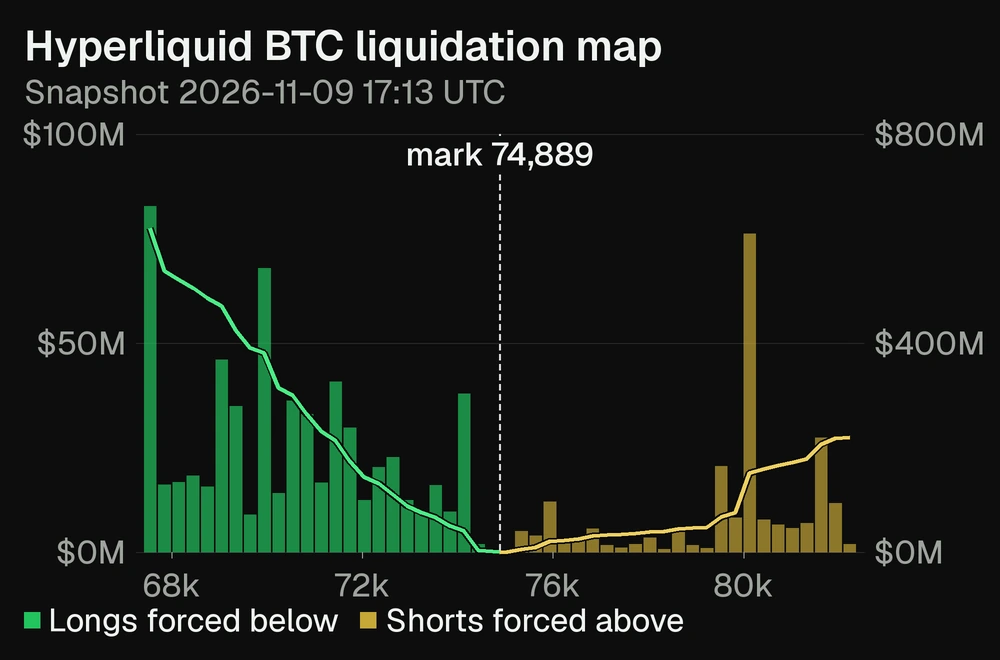
Each bar is one price bucket, about $300 wide. Green bars are long positions projected to be forced if the price falls to that bucket, read on the left axis. Gold bars are short positions forced if it rises there. The two lines, read on the right axis, add the buckets up from the mark outward, so they show how much would be forced along the way.
Projected forced-liquidation notional by price, Hyperliquid BTC, snapshot 9 Nov 2026 17:13 UTC, 50 buckets across 10% either side of the mark.
How to read this snapshot:
Close to the mark it is thin. Within 1% there were $40 million of longs below and $5 million of shorts above.
Longs outweigh shorts at every distance. Within 5%: $230 million of longs against $40 million of shorts.
The biggest long clusters sat near $67,550 ($82.7 million across 287 positions) and $69,950 ($67.9 million across 287 positions).
One short cluster stands out: $76.1 million near $80,130, held by only 50 positions, so a few large accounts.
The 48-hour BTC liquidation heatmap
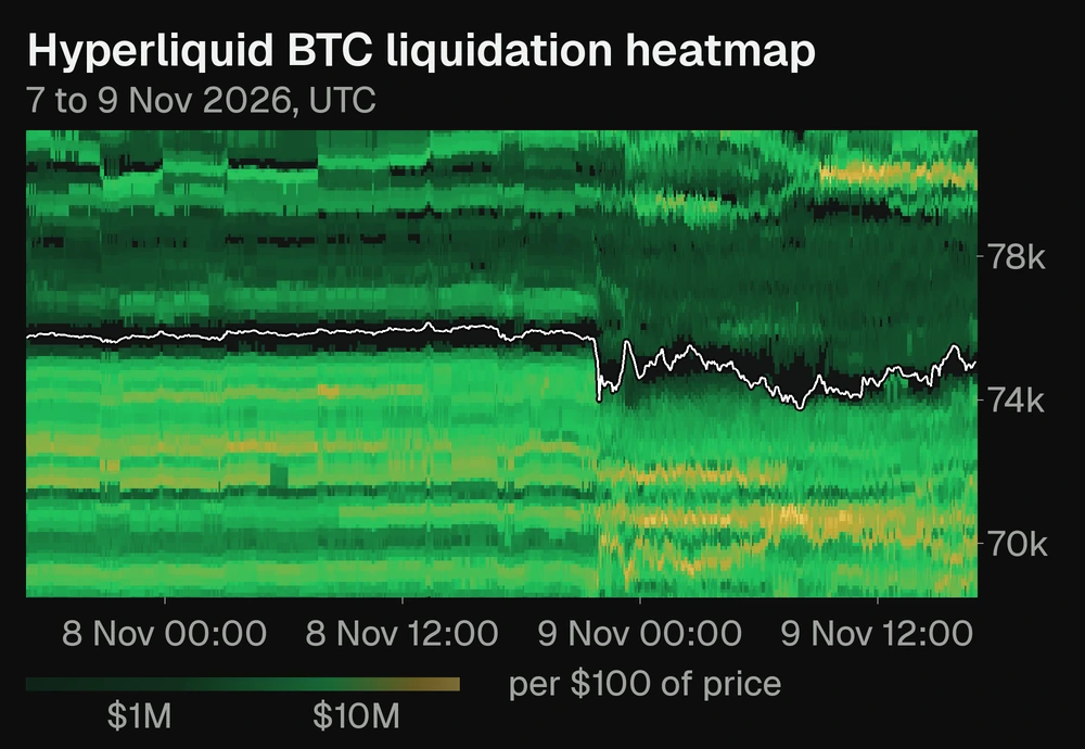
The heatmap stacks 576 snapshots side by side. Time runs left to right and price runs bottom to top. Brighter cells hold more notional that would be forced at that price, measured per $100 of price on a log scale. The white line is the mark price.
Projected forced-liquidation notional per $100 of price, Hyperliquid BTC, 576 snapshots from 7 Nov 17:03 to 9 Nov 16:58 UTC.
A dark gap follows the mark. A position whose forced-liquidation level reaches the mark is closed, so little exposure stays right next to the price.
The bands moved with the price. The densest long band sat near $72,800 at the start and near $70,000 at the end, after BTC fell $1,776 in the hour to 21:58 UTC on 8 November.
Exposure grew on both sides. Longs within 10% below the mark rose from $499 million to $567 million over the two days, and shorts above from $174 million to $222 million. A short band formed near $80,000.
A bright band is exposure, not a forecast. It says how much would be forced if the price got there, not that the price will. It changes as traders add margin, close positions or open new ones, which is why the snapshots repeat every 5 minutes.
range_pct sets how far either side of the mark to look (1 to 50%), and buckets how many price buckets to split it into (10 to 200). This Python walks out from the mark and prints what the map above shows:
import os

import requests

H = {"X-API-Key": os.environ["OXARCHIVE_API_KEY"]}
URL = "https://api.0xarchive.io/v1/hyperliquid/liquidations/BTC/levels"
snap = requests.get(URL, headers=H, params={"range_pct": 10, "buckets": 50}).json()["data"]

mark = snap["mid_price"]
print(snap["snapshot_ts"], "UTC, mark", f"{mark:,.0f}")

# Walk outward from the mark and add up what would be forced at each step.
below = sorted((b for b in snap["levels"] if b["price"] < mark), key=lambda b: -b["price"])
above = sorted((b for b in snap["levels"] if b["price"] > mark), key=lambda b: b["price"])
for pct in (1, 2, 5, 10):
    longs = sum(b["long_notional"] for b in below if b["price"] >= mark * (1 - pct / 100))
    shorts = sum(b["short_notional"] for b in above if b["price"] <= mark * (1 + pct / 100))
    print(f"within {pct:>2}%: longs below ${longs / 1e6:,.0f}M, shorts above ${shorts / 1e6:,.0f}M")

for side, rows in (("long", below), ("short", above)):
    top = sorted(rows, key=lambda b: -b[f"{side}_notional"])[:3]
    print(f"largest {side} buckets:",
          ", ".join(f"{b['price']:,.0f} (${b[side + '_notional'] / 1e6:,.1f}M, {b[side + '_count']} positions)" for b in top))
print("whole book: longs", f"${snap['total_long'] / 1e9:,.2f}B,", "shorts", f"${snap['total_short'] / 1e9:,.2f}B")
Output on 9 November 2026:
2026-11-09 17:13:24.000 UTC, mark 74,889
within  1%: longs below $40M, shorts above $5M
within  2%: longs below $66M, shorts above $23M
within  5%: longs below $230M, shorts above $40M
within 10%: longs below $620M, shorts above $220M
largest long buckets: 67,550 ($82.7M, 287 positions), 69,946 ($67.9M, 287 positions), 69,048 ($46.0M, 395 positions)
largest short buckets: 80,131 ($76.1M, 50 positions), 81,629 ($27.4M, 122 positions), 79,532 ($20.5M, 30 positions)
whole book: longs $1.26B, shorts $1.26B
Build the liquidation heatmap in Python
The history route returns up to 100 snapshots per request, oldest first, with a cursor for the next page. Each snapshot's buckets are centred on its own mark, so the script spreads every bucket over a fixed $100 price grid before drawing. It needs requests, numpy and matplotlib.
import os
from datetime import datetime

import matplotlib.pyplot as plt
import numpy as np
import requests

H = {"X-API-Key": os.environ["OXARCHIVE_API_KEY"]}
URL = "https://api.0xarchive.io/v1/hyperliquid/liquidations/BTC/levels/history"
params = {"start": "2026-11-07T17:00:00Z", "end": "2026-11-09T17:00:00Z",
          "limit": 100, "range_pct": 10, "buckets": 50}

snaps = []
while True:
    page = requests.get(URL, headers=H, params=params).json()
    snaps += page["data"]
    if not page["meta"].get("next_cursor"):
        break
    params["cursor"] = page["meta"]["next_cursor"]
print(len(snaps), "snapshots", snaps[0]["snapshot_ts"], "to", snaps[-1]["snapshot_ts"])

# One fixed $100 price grid for the whole window. Each snapshot's buckets are
# centred on its own mark, so split every bucket across the rows it overlaps.
STEP = 100
lo = min(s["levels"][0]["price"] for s in snaps) - 500
hi = max(s["levels"][-1]["price"] for s in snaps) + 500
edges = np.arange(lo, hi + STEP, STEP)
longs = np.zeros((len(edges) - 1, len(snaps)))
shorts = np.zeros_like(longs)
for j, s in enumerate(snaps):
    lv = s["levels"]
    width = lv[1]["price"] - lv[0]["price"]
    for b in lv:
        a, z = b["price"] - width / 2, b["price"] + width / 2
        i0, i1 = np.searchsorted(edges, a) - 1, np.searchsorted(edges, z)
        for i in range(max(i0, 0), min(i1, len(edges) - 1)):
            share = (min(z, edges[i + 1]) - max(a, edges[i])) / width
            longs[i, j] += b["long_notional"] * share
            shorts[i, j] += b["short_notional"] * share

times = [datetime.fromisoformat(s["snapshot_ts"]) for s in snaps]
mark = [s["mid_price"] for s in snaps]
fig, ax = plt.subplots(figsize=(11, 5))
rows = edges[:-1] + STEP / 2
ax.pcolormesh(times, rows, np.log10(longs + shorts + 1), cmap="YlGn_r", shading="nearest")
ax.plot(times, mark, color="white", lw=1)
ax.set_ylim(min(mark) * 0.93, max(mark) * 1.07)
ax.set_title("Hyperliquid BTC: projected forced-liquidation notional by price")
fig.savefig("btc_liquidation_heatmap.png", dpi=150, bbox_inches="tight")

last = snaps[-1]
below = sum(b["long_notional"] for b in last["levels"])
above = sum(b["short_notional"] for b in last["levels"])
top_long = max(last["levels"], key=lambda b: b["long_notional"])
top_short = max(last["levels"], key=lambda b: b["short_notional"])
print(f"latest mark {last['mid_price']:,.0f}: longs within 10% below ${below/1e6:,.0f}M, "
      f"shorts within 10% above ${above/1e6:,.0f}M")
print(f"largest long bucket {top_long['price']:,.0f} (${top_long['long_notional']/1e6:,.1f}M), "
      f"largest short bucket {top_short['price']:,.0f} (${top_short['short_notional']/1e6:,.1f}M)")
np.savez("grid.npz", longs=longs, shorts=shorts, edges=edges,
         times=np.array([t.timestamp() for t in times]), mark=np.array(mark))
Output on 9 November 2026:
576 snapshots 2026-11-07 17:03:17.000 to 2026-11-09 16:58:21.000
latest mark 75,050: longs within 10% below $567M, shorts within 10% above $222M
largest long bucket 70,097 ($50.7M), largest short bucket 80,003 ($47.6M)
Pass summary=true to get only the totals per snapshot, which is lighter when you are scanning a long window before choosing which snapshots to draw. For more ways to chart the same response, such as distance from the mark or notional per position, see five charts from projected Hyperliquid forced-liquidation levels.
What each field means
Field
Meaning
snapshot_ts
UTC time the snapshot was computed. Use it to order and align snapshots.
mid_price
Mark price at that time, the centre of the buckets.
levels[].price
Centre price of one bucket.
long_notional, short_notional
USD notional of long or short positions projected to be forced in that bucket.
long_count, short_count
How many positions make up that notional.
total_long, total_short
Notional across the whole book, not only the buckets returned. On 9 November both were $1.26 billion for BTC.
flagged_notional
Notional counted in the totals but computed approximately or not placed in a returned bucket.
block_number
The Hyperliquid block the computation started from, typically 30 to 65 minutes before snapshot_ts. Positions are then rolled forward with every fill up to snapshot_ts.
Swap BTC for any Hyperliquid perpetual. At 17:18 UTC on 9 November, ETH showed $216 million of longs within 10% below its mark and $23 million of shorts above; HYPE showed $332 million and $270 million. For HIP-3 markets, use /v1/hyperliquid/hip3/liquidations/{symbol}/levels and keep the builder prefix and case, for example xyz:TSLA. HIP-3 cross-margined exposure is reported in flagged_notional rather than in the buckets.
Liquidations that already happened
Everything above is projected exposure. Completed forced liquidations are a separate dataset: one row per liquidation, with price, size and side. The Hyperliquid liquidations data guide covers it, and our open-source notebook turns it into a heatmap of past liquidations, cascade detection and a long versus short balance over time. Its 3-day example counted 13,399 liquidations worth $143 million. For a heatmap of resting orders rather than positions, see the Hyperliquid order book heatmap guide.
Questions
How often does the Hyperliquid liquidation heatmap update?
About every 5 minutes since 13 August 2026, and about every 45 minutes from 27 July to 13 August 2026.
Is this a liquidation price for my own position?
No. It groups every account's projected forced-liquidation level into price buckets. It does not return any one account's liquidation price.
Which plan do I need?
Both routes work on every plan and cost more credits per request than standard routes. The Free plan reads the last 30 days; Build and above read everything from 27 July 2026. See pricing.