Five charts from projected Hyperliquid...

A liquidation heatmap is useful, but it is not the only way to read projected forced-liquidation price-level history. This guide uses one real 48-hour BTC response to show where projected long- and short-side notional sits, how it accumulates, how position counts change by bucket and how distance-band clusters move over time.

What this is: a view of projected forced-liquidation price levels from the history endpoint. What this is not: a record of completed forced executions or a map of pending take-profit and stop-loss triggers. Those are separate datasets.

GET /v1/hyperliquid/liquidations/BTC/levels/history
  ?start=1788117625413
  &end=1788290425413
  &limit=100
  &range_pct=10
  &buckets=50

Each snapshot includes snapshot_ts, block_number, mid_price, total_long, total_short, flagged_notional and price buckets with long_notional, short_notional, long_count and short_count.

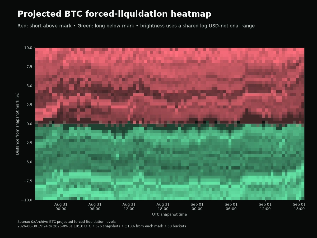
1. Projected forced-liquidation heatmap

Normalize each bucket by its distance from that snapshot's mid_price, then place time on the horizontal axis. Red cells show short positions projected to liquidate above the mark. Green cells show long positions projected to liquidate below the mark. Brightness uses the same log-scaled USD-notional range on both sides.

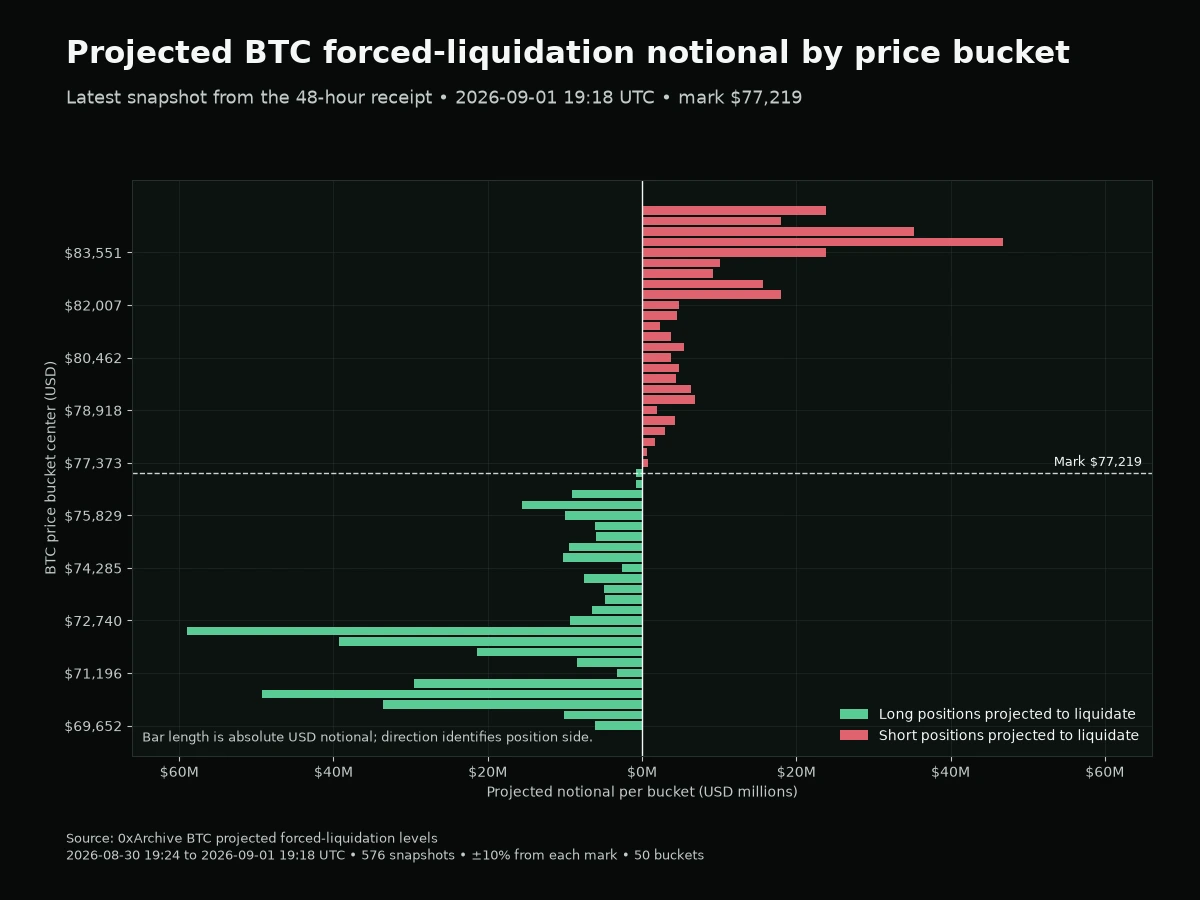
Heatmap of projected BTC forced-liquidation notional over 48 hours, with short-side levels above the mark in red and long-side levels below the mark in green — Projected BTC forced-liquidation notional by snapshot time and distance from the mark. Open the full-resolution chart.

2. Projected notional by price bucket

Take the latest snapshot and plot each bucket at its center price. Long-side projected notional extends left and short-side projected notional extends right. The dashed line marks the snapshot's mid_price.

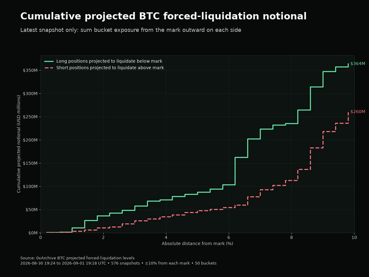
Horizontal price ladder of projected BTC forced-liquidation notional, with long positions below the mark and short positions above the mark — Latest projected BTC forced-liquidation notional by price bucket. Open the full-resolution chart.

3. Cumulative projected notional

Sort the latest snapshot by absolute distance from mid_price, then sum projected notional outward. The result shows how much long-side exposure sits below the mark and how much short-side exposure sits above it as the distance widens.

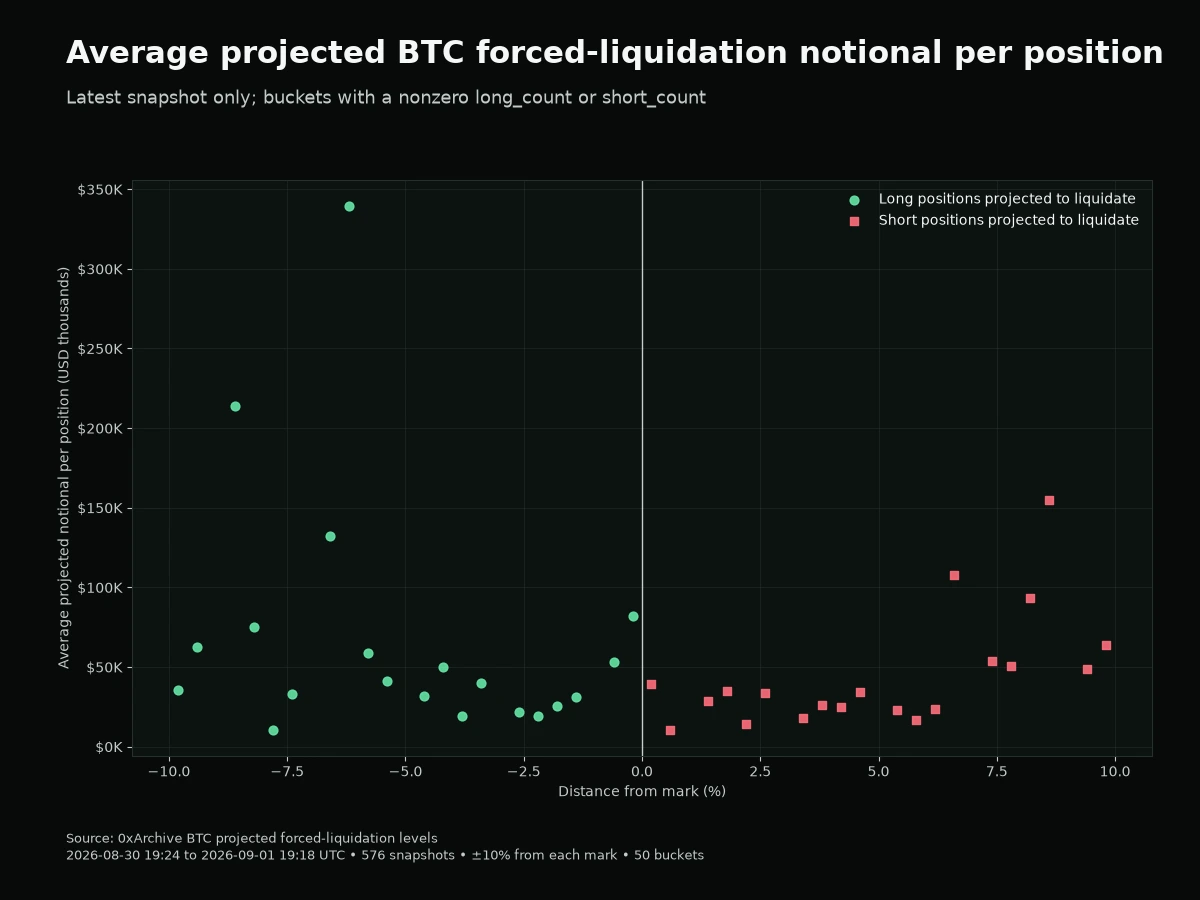
Cumulative projected BTC forced-liquidation notional as distance from the mark widens, comparing long positions below the mark with short positions above it — Cumulative projected BTC forced-liquidation notional from the mark outward. Open the full-resolution chart.

4. Average projected notional per position

Notional alone cannot distinguish many smaller positions from a smaller number of larger ones. For buckets with nonzero counts, divide long_notional by long_count and short_notional by short_count.

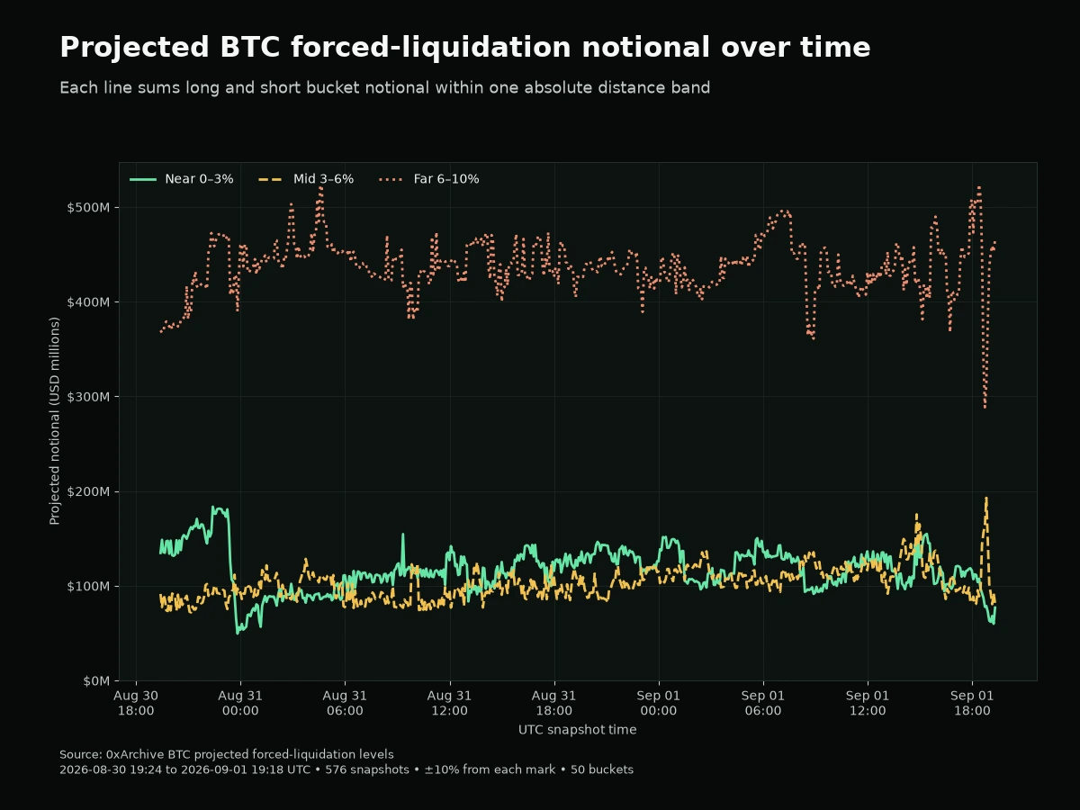
Average projected BTC forced-liquidation notional per position by distance from the mark, with long-side circles and short-side squares — Average projected BTC forced-liquidation notional per position in the latest snapshot. Open the full-resolution chart.

5. Distance-band movement over time

For every snapshot, sum long- and short-side projected notional into three absolute distance bands: 0–3%, 3–6% and 6–10% from mid_price. This separates changes near the mark from shifts farther away.

Projected BTC forced-liquidation notional over 48 hours grouped into near, mid and far distance bands from the mark — Projected BTC forced-liquidation notional over time by absolute distance from the mark. Open the full-resolution chart.

Build all five charts from one response

{
  "snapshot_ts": "2026-08-30 19:24:31.000",
  "block_number": 1129510000,
  "mid_price": 78910.0,
  "total_long": 1156845230.97,
  "total_short": 1111012990.69,
  "flagged_notional": 217914673.56,
  "levels": [
    {
      "price": 71176.82,
      "long_notional": 15710644.53,
      "short_notional": 0.0,
      "long_count": 313,
      "short_count": 0
    }
  ]
}

Group the bucket rows by price, long or short side, position count, distance from mid_price or snapshot_ts, depending on the chart. The response stays the same.

For exact endpoint fields and parameters, see the projected forced-liquidation level history reference. For completed forced executions, use the completed liquidation-events guide. Pending take-profit and stop-loss concentrations use the separate trigger-level history contract.